FLUX.1-dev with Diffuse: Modular Sampling Framework#
This notebook demonstrates how to use FLUX.1-dev [Labs, 2024] with the Diffuse sampling framework - showcasing how a modular sampling framework can help understand, investigate and experiment with sota pre-trained models.
A lot of exciting diffusion research isn’t about training models - it’s about the algorithms built on top:
🎨 Image editing (InstructPix2Pix, DiffEdit, Imagic)
🖼️ Inpainting & outpainting (RePaint, Blended Diffusion)
🔍 Inverse problems (DPS, RED-diff, medical imaging)
🎯 Controllable generation (ControlNet-style, regional control)
📐 Novel sampling methods (better integrators, adaptive schedules)
🧠 Bayesian Experimental Design (adaptive sampling for inverse problems)
All of these need modular sampling infrastructure to test, iterate and experiment with each component separately. Because it is hard to change different components of the pipeline (the integrator, the discretization schedule or the conditionning) most researchers tend to stick to one setting only for their experiments.
Diffuse solves this: Load pre-trained models → Choose your components → Assess the impact of each component on your research.
What We’ll Explore#
Flow Matching Models - Understanding FLUX as a velocity field predictor
Modular Components - Swap timers, integrators, guidance without touching model code
Quality Comparisons - Visual side-by-side across configurations
What is FLUX.1-dev?#
FLUX.1-dev [Labs, 2024] is a state-of-the-art text-to-image model trained using flow matching [Liu et al., 2023] [Lipman et al., 2022] (also called rectified flow). Unlike traditional diffusion models that learn to denoise images, FLUX learns a velocity field that transforms noise into images along straight paths.
Flow Matching Background#
As detailed in the Diffusion Crash Course, flow matching uses the straight-line interpolation path:
where \(x_0\) is clean data and \(\varepsilon\) is Gaussian noise. FLUX [Labs, 2024] learns a velocity field \(v_\theta(x_t, t, c)\) conditioned on text embeddings \(c\) that defines the flow ODE (see Eq. (8) in the crash course):
In this context, Diffuse allows you to:
✅ Swap integrators (Euler, Heun, DPM++, DDIM) without retraining
✅ Change discretization schedules (uniform, adaptive, learned)
✅ Add stochasticity (churning, noise injection) for diversity
✅ Apply to inverse problems (inpainting, super-resolution, deblurring)
✅ Compose guidance methods (classifier-free)
Diffuse makes this modular and easy. Just load weights and experiment with sampling.
Setup#
JAX devices: [CudaDevice(id=0)]
Configuration#
Set the HuggingFace repo and generation parameters. The tutorial downloads the FLUX jax checkpoint from jcopo/flux_jax automatically, so no manual path configuration is required.
# HuggingFace model source
HF_REPO_ID = "jcopo/flux_jax"

CHECKPOINT_DIR = Path(
    snapshot_download(
        repo_id=HF_REPO_ID,
        repo_type="model",
    )
)
print(f"Using checkpoint from: {CHECKPOINT_DIR}")

# Generation parameters
PROMPT = "A serene landscape with mountains at sunset, highly detailed, photorealistic"
HEIGHT = 512
WIDTH = 512
NUM_STEPS = 20
GUIDANCE_SCALE = 4.0
SEED = 42

print(f"Prompt: {PROMPT}")
print(f"Resolution: {WIDTH}x{HEIGHT}")
print(f"Steps: {NUM_STEPS}")
Using checkpoint from: /linkhome/rech/genini01/upd68za/.cache/huggingface/hub/models--jcopo--flux_jax/snapshots/2421c1312395408de2fdd391fe5c0bb616363c6f
Prompt: A serene landscape with mountains at sunset, highly detailed, photorealistic
Resolution: 512x512
Steps: 20
Load FLUX Model#
This section demonstrates Diffuse’s separation of concerns - one of the key design principles that enables rapid experimentation.
The Three Stages#
Model Loading -
FluxModelLoaderhandles checkpoints, tokenizers, text encodersText Conditioning -
prepare_conditioned_networkencodes prompt, returns conditioned velocity fieldSampling - Modular components (Timer, Integrator, Denoiser) handle generation
What does prepare_conditioned_network do?#
FLUX was trained using flow matching to predict velocity fields. This function:
Tokenizes your prompt using CLIP and T5 tokenizers
Encodes text through CLIP (pooled embeddings) and T5 (sequence embeddings)
Loads the FLUX transformer onto GPU
Returns a conditioned velocity field
v(x_t, t, c)- a function mapping (latents + time + prompt) → velocities
Think of it as “baking” your text prompt into the velocity field. Now you can sample from this field using any integrator without touching text encoders again.
This is quite interesting for Research:#
✅ Text encoders offloaded after encoding (saves memory)
✅ Clean velocity field interface for sampling experiments
✅ Swap sampling components without re-encoding
✅ Zero loading complexity for your research code
# Load model
loader = FluxModelLoader(checkpoint_dir=CHECKPOINT_DIR, verbose=True)

# Prepare conditioned velocity field
conditioned = loader.prepare_conditioned_network(
    prompt=PROMPT,
    negative_prompt=None,
    guidance_scale=GUIDANCE_SCALE,
    height=HEIGHT,
    width=WIDTH,
)

print(f"\nConditioned network ready (dtype={conditioned.dtype})")
[flux-loader] Host CPU device: cpu:0
[flux-loader] Active compute device: gpu:0
[flux-loader] Preparing conditioned network
[flux-loader] Encoding 1 prompt(s)
[flux-loader] Tokenizing prompts for CLIP/T5
[flux-loader] Restoring clip_text on gpu:0
[flux-loader] Loaded clip_text parameters (~234.72MB)
[flux-loader] CLIP pooled embedding shape (1, 768), dtype=bfloat16
[flux-loader] Restoring t5_text on gpu:0
[flux-loader] Loaded t5_text parameters (~8.87GB)
[flux-loader] T5 hidden state shape (1, 512, 4096), dtype=bfloat16
[flux-loader] Releasing text encoders
[flux-loader] Releasing clip_text from gpu:0
[flux-loader] Releasing t5_text from gpu:0
[flux-loader] Restoring transformer on gpu:0
[flux-loader] Loaded transformer parameters (~22.17GB)

Conditioned network ready (dtype=bfloat16)
Helper Functions: Modular Sampling with Diffuse#
The key to Diffuse’s power is separation of concerns. Each component has one job:
Timer: Decides WHEN to evaluate the model (discretization schedule)
Predictor: Wraps the velocity field
v(x_t, t)from FLUX so that it can be evaluated as both velocity, score or noiseIntegrator: Decides HOW to step from
x_ttox_{t-1}(numerical ODE solver)Denoiser: Orchestrates the full sampling loop
This modularity is the entire point: change one component, everything else stays the same.
Want to test a new integrator idea? Just swap one line.
Want to try a different schedule? Just swap one line.
Want to add guidance? Just swap the Denoiser.
def run_generation(
    conditioned_network: FluxConditionedNetwork,
    timer,
    integrator_class,
    num_steps: int,
    seed: int,
) -> jax.Array:
    """Generate image using modular Diffuse components."""
    # Modular component assembly
    flow = Flow(tf=1.0)
    predictor = Predictor(
        model=flow,
        network=conditioned_network.network_fn,
        prediction_type="velocity",
    )
    integrator = integrator_class(model=flow, timer=timer)
    denoiser = Denoiser(
        integrator=integrator,
        model=flow,
        predictor=predictor,
        x0_shape=(transformer_hw[0], transformer_hw[1], conditioned_network.in_channels),
    )

    # Run sampling
    key = jax.random.PRNGKey(seed)
    state, _ = denoiser.generate(
        rng_key=key,
        n_steps=num_steps,
        n_particles=1,
        keep_history=False,
    )
    return state.integrator_state.position
Part 1: Timer Comparison#
Timers control the time discretization \(t \in [0, 1]\). Different schedules allocate more steps to different noise levels.
VpTimer#
Linear discretization: \(t_i = t_f + \frac{i}{N}(\epsilon - t_f)\)
FluxTimer#
Applies a Möbius transformation to bias sampling toward low-noise regions:
Static mode: Fixed \(\mu = 1.15\) (FLUX default)
Dynamic mode: Resolution-adaptive \(\mu(L)\) based on sequence length \(L\)
The Möbius shift allocates more steps to fine details (low noise), improving quality.
# Create timers
vp_timer = VpTimer(n_steps=NUM_STEPS, eps=1e-3, tf=1.0)
flux_timer_static = FluxTimer(n_steps=NUM_STEPS, eps=1e-3, tf=1.0, shift=1.15, use_dynamic_shift=False)
flux_timer_dynamic = FluxTimer(n_steps=NUM_STEPS, eps=1e-3, tf=1.0, shift=1.15, use_dynamic_shift=True)
_, transformer_hw = _latent_shapes(HEIGHT, WIDTH)
image_seq_len = transformer_hw[0] * transformer_hw[1]
flux_timer_dynamic.set_image_seq_len(image_seq_len)
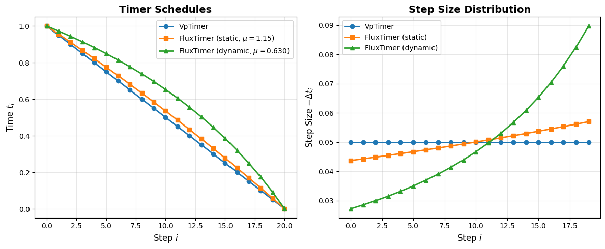
Resolution: 512x512 → 1024 tokens
Dynamic shift μ: 0.630
Generate with Different Timers#
We use DDIMIntegrator [Song et al., 2021] (see crash course section on DDIM) to isolate the effect of the timer.
print("Generating with VpTimer...")
latents_vp = run_generation(conditioned, vp_timer, DDIMIntegrator, NUM_STEPS, SEED)
img_vp = decode_and_display(latents_vp, loader)

print("Generating with FluxTimer (static)...")
latents_flux_static = run_generation(conditioned, flux_timer_static, DDIMIntegrator, NUM_STEPS, SEED)
img_flux_static = decode_and_display(latents_flux_static, loader)

print("Generating with FluxTimer (dynamic)...")
latents_flux_dynamic = run_generation(conditioned, flux_timer_dynamic, DDIMIntegrator, NUM_STEPS, SEED)
img_flux_dynamic = decode_and_display(latents_flux_dynamic, loader)

timer_images = {
    "VpTimer": img_vp,
    "FluxTimer (Static)": img_flux_static,
    "FluxTimer (Dynamic)": img_flux_dynamic,
}

plot_comparison(
    timer_images,
    f"Timer Comparison (DDIM, {NUM_STEPS} steps)",
    figsize=(18, 6),
)
Generating with VpTimer...
[flux-loader] Decoding latents through VAE
[flux-loader] Restoring vae on gpu:0
[flux-loader] Loaded vae parameters (~319.75MB)
[flux-loader] Releasing VAE
[flux-loader] Releasing vae from gpu:0
Generating with FluxTimer (static)...
[flux-loader] Decoding latents through VAE
[flux-loader] Restoring vae on gpu:0
[flux-loader] Loaded vae parameters (~319.75MB)
[flux-loader] Releasing VAE
[flux-loader] Releasing vae from gpu:0
Generating with FluxTimer (dynamic)...
[flux-loader] Decoding latents through VAE
[flux-loader] Restoring vae on gpu:0
[flux-loader] Loaded vae parameters (~319.75MB)
[flux-loader] Releasing VAE
[flux-loader] Releasing vae from gpu:0
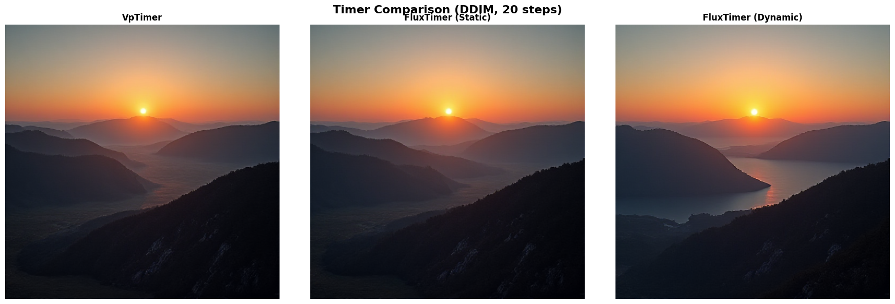
Expected Differences:
VpTimer: Uniform steps, may miss fine details
FluxTimer (Static): More low-noise steps, better details
FluxTimer (Dynamic): Adapts to the resolution of the image, see the finer details in the lake
Part 2: Integrator Comparison#
What Are Integrators?#
FLUX gives us a velocity field v(x_t, t) - it tells us “which direction to move” at each point. An integrator is the numerical method we use to follow that velocity field from noise (t=1) to image (t=0). It is defined by an Integrator class that implements how to go from x_t to x_{t-1}.
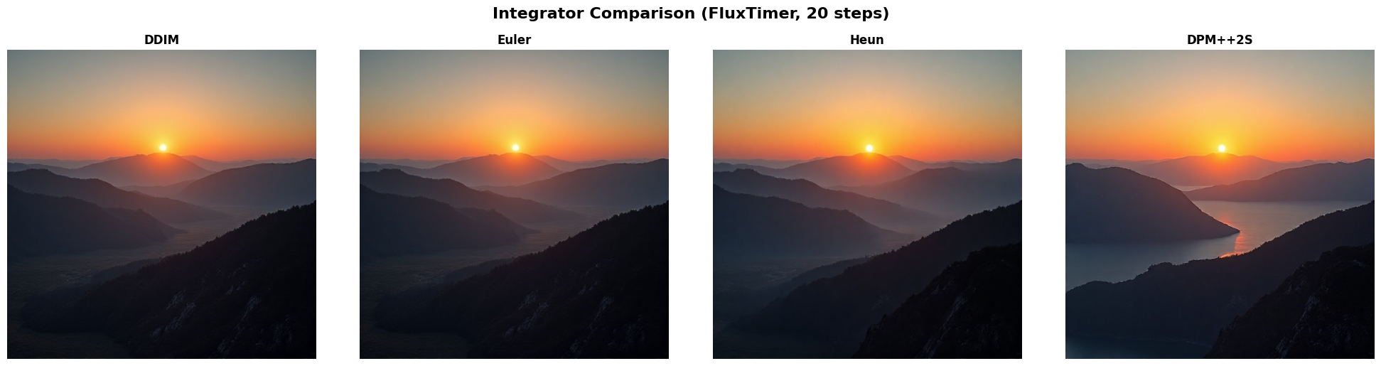
Why Integrators Matter for Quality#
Different integrators can significantly affect visual quality. For example:
DPM++2S often produces sharper reflections (like sunlight on water)
Heun preserves fine texture details better than Euler
Integrators We’ll Compare#
DDIM [Song et al., 2021] (see crash course section on DDIM)
Fast, deterministic, well-tested
Good default choice for most applications
Euler (First-Order)
Simplest: just follow the velocity directly
Fast but can accumulate errors over many steps
Good for quick previews
Heun (Second-Order)
“Look ahead” method: predicts next step, corrects itself
2x slower (two model evaluations per step) but more accurate
Better detail preservation
DPM++2S [Lu et al., 2022] (Second-Order Optimized)
Like Heun but with optimized stability
Often produces best quality
Key Insight: Quality vs Speed Trade-off#
Same steps: Heun ≈ DPM++2S > DDIM > Euler (quality)
Same compute: DDIM at 40 steps ≈ Heun at 20 steps
For FLUX: DPM++2S often produces noticeably better fine details
Let’s see the visual differences using FluxTimer. Diffuse allows you to test different integrators with the same code, with minimal friction in code changes:
# Use FluxTimer for fair comparison
timer_for_comparison = FluxTimer(n_steps=NUM_STEPS, eps=1e-3, tf=1.0, shift=1.15, use_dynamic_shift=False)

integrators = [
    ("DDIM", DDIMIntegrator),
    ("Euler", EulerIntegrator),
    ("Heun", HeunIntegrator),
    ("DPM++2S", DPMpp2sIntegrator),
]

integrator_images = {}

for name, integrator_class in integrators:
    print(f"Generating with {name}...")
    latents = run_generation(conditioned, timer_for_comparison, integrator_class, NUM_STEPS, SEED)
    img = decode_and_display(latents, loader)
    integrator_images[name] = img
Generating with DDIM...
[flux-loader] Decoding latents through VAE
[flux-loader] Restoring vae on gpu:0
[flux-loader] Loaded vae parameters (~319.75MB)
[flux-loader] Releasing VAE
[flux-loader] Releasing vae from gpu:0
Generating with Euler...
[flux-loader] Decoding latents through VAE
[flux-loader] Restoring vae on gpu:0
[flux-loader] Loaded vae parameters (~319.75MB)
[flux-loader] Releasing VAE
[flux-loader] Releasing vae from gpu:0
Generating with Heun...
[flux-loader] Decoding latents through VAE
[flux-loader] Restoring vae on gpu:0
[flux-loader] Loaded vae parameters (~319.75MB)
[flux-loader] Releasing VAE
[flux-loader] Releasing vae from gpu:0
Generating with DPM++2S...
[flux-loader] Decoding latents through VAE
[flux-loader] Restoring vae on gpu:0
[flux-loader] Loaded vae parameters (~319.75MB)
[flux-loader] Releasing VAE
[flux-loader] Releasing vae from gpu:0
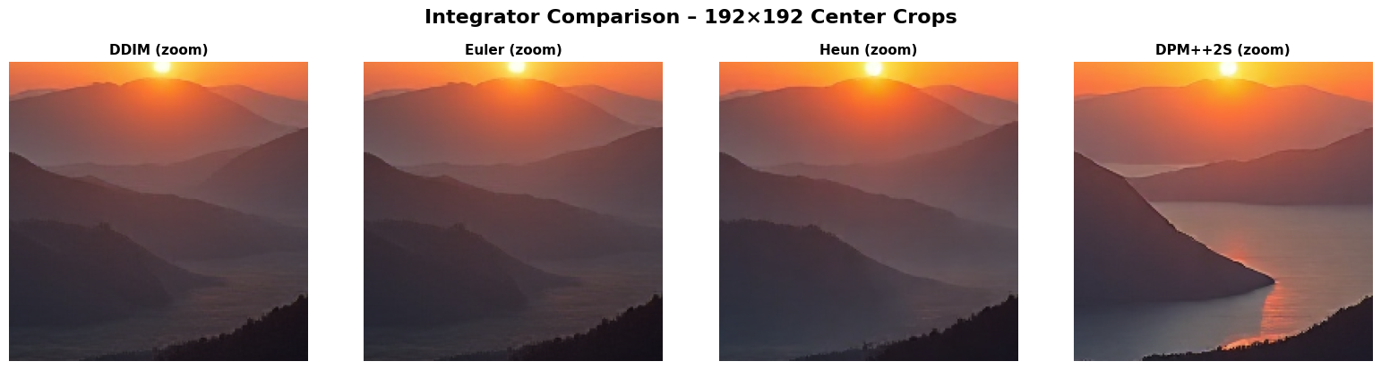
Integrator Detail Zooms#
To highlight subtle differences, we also compare center crops from each integrator output. This makes sheen, edge contrast, and texture preservation easier to inspect.
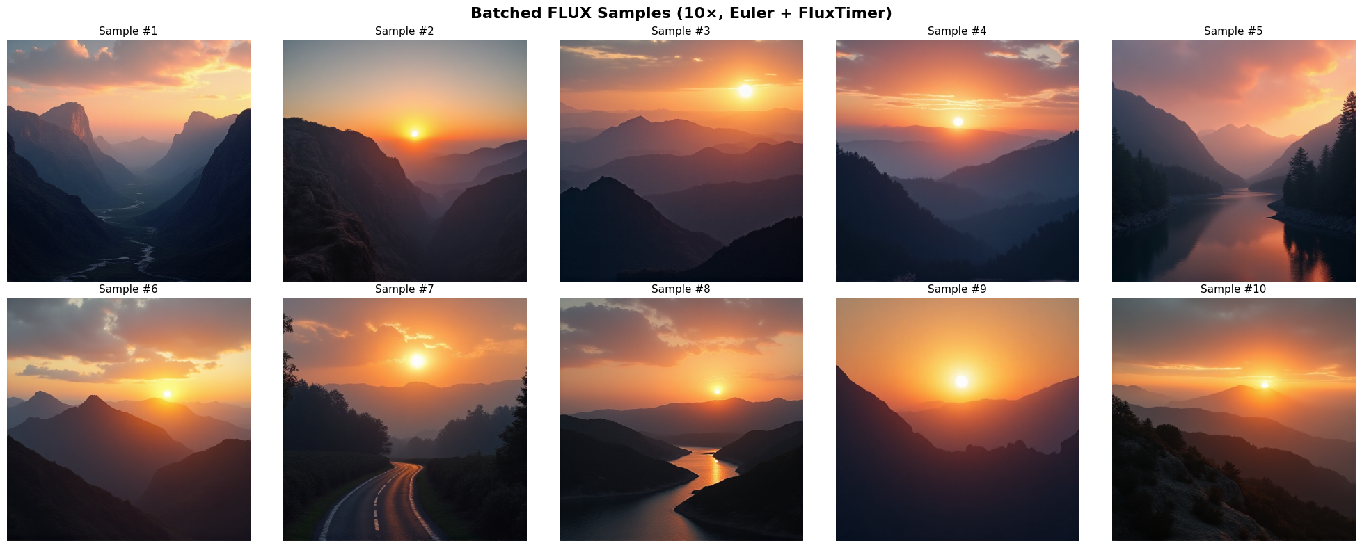
Part 3: Batched Generation Benchmark#
Because .generate() is JAX-powered, specifying n_particles enables us to draw many samples in parallel (10 in this example). JAX handles this efficiently by using vmap under the hood to maximize GPU utilization.
import time

NUM_BENCHMARK_SAMPLES = 10
benchmark_seed = SEED + 1234

flow = Flow(tf=1.0)
predictor = Predictor(
    model=flow,
    network=conditioned.network_fn,
    prediction_type="velocity",
)
integrator = EulerIntegrator(model=flow, timer=flux_timer_dynamic)

benchmark_denoiser = Denoiser(
    integrator=integrator,
    model=flow,
    predictor=predictor,
    x0_shape=(
        transformer_hw[0],
        transformer_hw[1],
        conditioned.in_channels,
    ),
)

key_benchmark = jax.random.PRNGKey(benchmark_seed)
start_time = time.perf_counter()
benchmark_state, _ = benchmark_denoiser.generate(
    rng_key=key_benchmark,
    n_steps=NUM_STEPS,
    n_particles=NUM_BENCHMARK_SAMPLES,
    keep_history=False,
)

benchmark_latents = benchmark_state.integrator_state.position
benchmark_images = loader.decode_latents(benchmark_latents)
benchmark_images.block_until_ready()
generation_time = time.perf_counter() - start_time

print(f"✓ Generated {NUM_BENCHMARK_SAMPLES} samples in {generation_time:.2f}s ")
Summary: The Power of Modular Sampling#
An interesting direction for diffusion research lies in algorithms built on top of pre-trained models. Diffuse enables you to:
Focus on research – minimal setup overhead, intuitive pipeline
Build on SOTA – seamless integration with FLUX, Stable Diffusion, and custom models
Prototype fast – from idea to working code in under 50 lines
Built for Sampling Research This notebook demonstrates Diffuse’s core philosophy: separation of concerns enables rapid experimentation. It provides clean protocols to implement new ideas on:
Novel ODE/SDE solvers via the Integrator protocol
Adaptive schedules via the Timer protocol
Guidance methods by extending Denoiser
Inverse problems via ForwardModel implementations
What We Explored#
FLUX as Flow Matching – velocity field prediction via continuous normalizing flows (see Eq. (7) in the crash course)
Timers – discretization schedules including VpTimer and FluxTimer with Möbius shift
Integrators – ODE solvers (DDIM, Euler, Heun, DPM++2S)
Batched Sampling – parallel 10-sample generation
References#
Yaron Lipman, Ricky T. Q. Chen, Heli Ben-Hamu, Maximilian Nickel, and Matt Le. Flow matching for generative modeling. arXiv preprint arXiv:2210.02747, 2022.
Xingchao Liu, Chengyue Gong, and Qiang Liu. Flow straight and fast: learning to generate and transfer data with rectified flow. In International Conference on Learning Representations (ICLR). 2023.
Cheng Lu, Yuhao Zhou, Fan Bao, Jianfei Chen, Chongxuan Li, and Jun Zhu. Dpm-solver++: fast solver for guided sampling of diffusion probabilistic models. arXiv preprint arXiv:2211.01095, 2022.