Diffusion Models on MNIST: A Comprehensive Tutorial

Diffusion Models on MNIST: A Comprehensive Tutorial#

Diffusion tutorial light enough to run on CPU. This tutorial demonstrates the whole pipeline, from how to download trained diffusion models from Hugging Face to setting up different integrators for generation and for solving inverse problems.

Loading Models from Hugging Face - Download and setup pretrained weights
Unconditional Generation - Generate MNIST digits from noise using different integrators availables in Diffuse: EulerMaruyamaIntegrator (stochastic first-order), DDIMIntegrator (deterministic first-order), HeunIntegrator (deterministic second-order), DPMpp2sIntegrator (optimized second-order).
Conditional Generation - Solve inverse problems (inpainting) using DPS (Diffusion Posterior Sampling)

Foreword on Diffuse#

Diffusion models learn to reverse a noise corruption process. The FlowModel class uses rectified flow [Liu et al., 2023] (a.k.a. flow matching) implementing the linear interpolation path

\[ x_t = (1 - t) x_0 + t \varepsilon, \quad \varepsilon \sim \mathcal{N}(0, I), \quad t \in [0, 1] \]

The learned velocity field will get loaded to the Predictor class and can be evaluated with predictor.velocity(x, t).

While we learn a velocity field, we can use the equivalances developed in the Diffusion Crash Course to convert the velocity field to a score function \(s_\theta(x_t, t)\) or to a noise prediction model \(\epsilon_\theta(x_t, t)\). This is done automatically in the Predictor classes and allows us to sample using integrators originally designed for score-based or noise prediction models, eg the DDIMIntegrator.

Building on top of the Integrator base class, CondDenoiser classes implement different conditional sampling strategies for solving inverse problems. In this tutorial, we will use the DPSDenoiser class implementing Diffusion Posterior Sampling (DPS) [Chung et al., 2023]. Even if originally designed for score-based models and DDIMIntegrator or EulerMaruyamaIntegrator, the DPSDenoiser class can be used with any integrator available in Diffuse and any interpolating path (eg rectified flow).

Setup and Model Loading#

First, we’ll set up the environment and download a pretrained model from Hugging Face.

Download Model from Hugging Face#

We’ll download the pretrained MNIST model from Hugging Face Hub. This model was trained using rectified flow and flow matching loss.

/Users/jacopoiollo/louvre/main/.venv/lib/python3.13/site-packages/tqdm/auto.py:21: TqdmWarning: IProgress not found. Please update jupyter and ipywidgets. See https://ipywidgets.readthedocs.io/en/stable/user_install.html
  from .autonotebook import tqdm as notebook_tqdm

Downloading model from HuggingFace Hub...
Model loaded successfully (CondUNet2D)

Setup Flow Model and Predictor#

We use a Flow (rectified flow) model with velocity prediction. The predictor converts between different parameterizations (score, noise, velocity, x0), allowing us to use any integrator regardless of its original formulation.

# Create Flow model (rectified flow)
flow = Flow()


# Create network wrapper
def network_fn(x, t):
    """Neural network velocity field v_θ(x,t)"""
    return model(x, t).output


# Create predictor with velocity prediction type
predictor = Predictor(model=flow, network=network_fn, prediction_type="velocity")

# Test model inference
key = jax.random.PRNGKey(42)
batch_size = 4
img_shape = (28, 28, 1)

# Create dummy input
dummy_x = jax.random.normal(key, (batch_size, *img_shape))
dummy_t = jnp.ones((batch_size,)) * 0.5

# Run model forward pass
output = model(dummy_x, dummy_t)
velocity = predictor.velocity(dummy_x[0], dummy_t[0])
score = predictor.score(dummy_x[0], dummy_t[0])

Unconditional Generation: Comparing Integrators#

We now will generate MNIST digits from pure noise using several numerical integrators, each solving the diffusion dynamics in a distinct way.

Euler–Maruyama: EulerMaruyamaIntegrator
A stochastic integrator that discretizes the reverse-time SDE, adding Gaussian noise at each step. It promotes diverse generations but may yield slightly blurrier samples.

DDIM: DDIMIntegrator
A deterministic reformulation of the diffusion sampling process [Song et al., 2021], removing stochasticity to produce consistent, high-quality samples with fewer denoising steps.

Heun: HeunIntegrator
A second-order Runge–Kutta (predictor–corrector) solver for the probability flow ODE, offering improved local accuracy and stability compared to first-order methods.

DPM++: DPMpp2sIntegrator
A family of multi-step solvers [Lu et al., 2022] that use adaptive step updates and midpoint prediction for fast, high-fidelity sampling, representing the current state of the art among diffusion ODE integrators.

We will compare the generations obtained from these integrators side by side.

# Setup common parameters
n_steps = 50
n_samples = 16

# VpTimer: Creates equidistant time discretization between 0 and 1 with n_steps
# eps is used to clip time for numerical stability near 0
timer = VpTimer(eps=1e-3, tf=1.0, n_steps=n_steps)

# Euler-Maruyama: Stochastic integrator
euler_maruyama = EulerMaruyamaIntegrator(model=flow, timer=timer)

# DDIM: Deterministic integrator
ddim = DDIMIntegrator(model=flow, timer=timer)

# Heun: Second-order deterministic integrator
heun = HeunIntegrator(model=flow, timer=timer)

# DPM++: Multi-step second-order deterministic integrator
dpmpp = DPMpp2sIntegrator(model=flow, timer=timer)

All integrators can be used interchangeably by simply changing the integrator argument in the Denoiser class. To generate samples, we simply call the generate method with a random key, number of steps, and number of samples. keep_history=True allows us to store intermediate states for visualization.

euler_denoiser = Denoiser(
    integrator=euler_maruyama,
    model=flow,  # The SDE/Flow model
    predictor=predictor,
    x0_shape=img_shape,
)
key_euler = jax.random.PRNGKey(456)
state_euler, history_euler = euler_denoiser.generate(key_euler, n_steps, n_samples, keep_history=True)

We’ve generated samples with Euler-Maruyama. Now let’s generate with the other integrators (DDIMIntegrator, HeunIntegrator, DPMpp2sIntegrator) and compare the results.

_images/1863b75da9954e2d83f9a3f2f28ae1f6308680831493caa661a698e6a7c69d2a.png

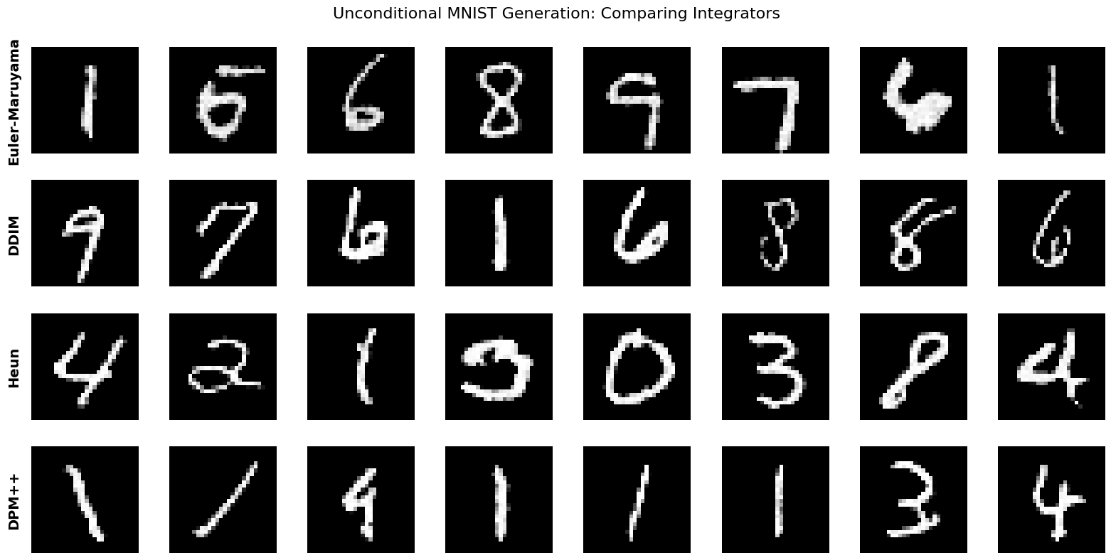
What to Look For: Unconditional Generation#

Euler-Maruyama: May show more variation between samples (stochastic)
DDIM: Should produce clean, sharp digits
Heun/DPM++: Often highest quality, smoothest gradients

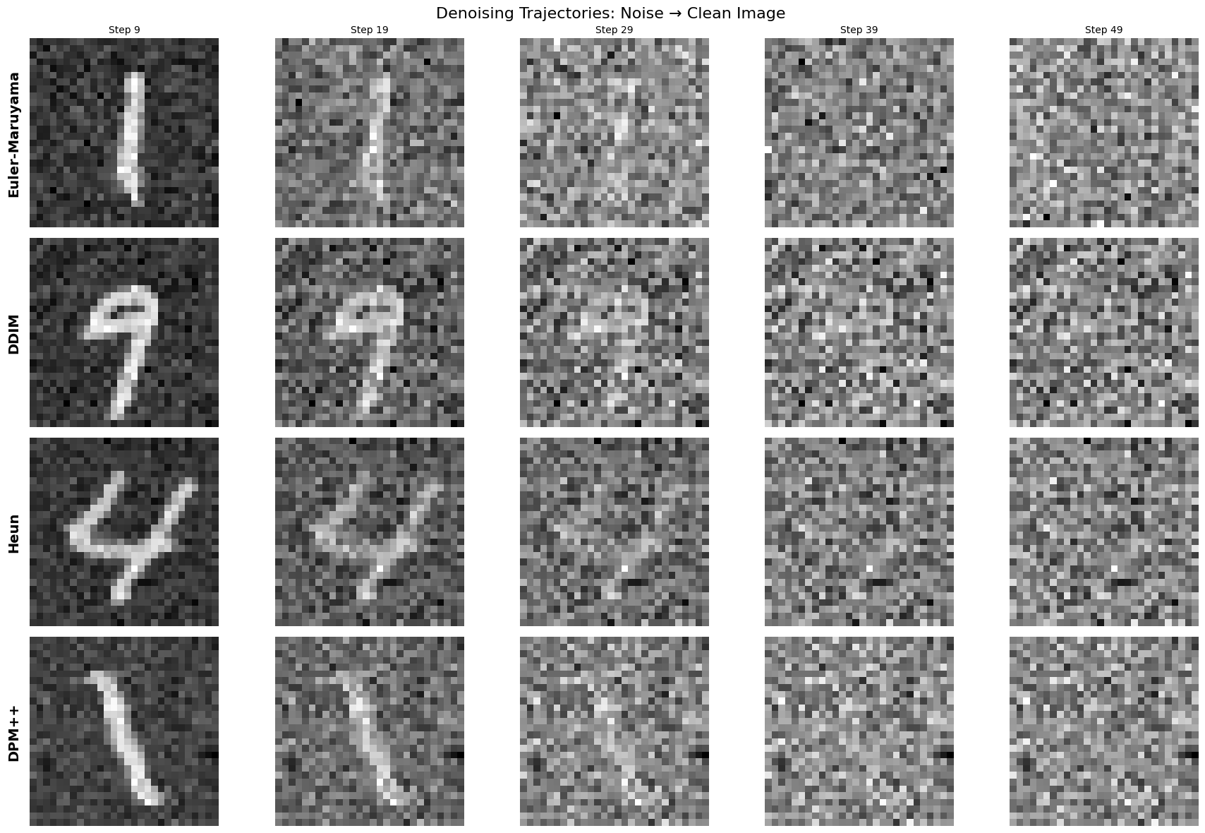
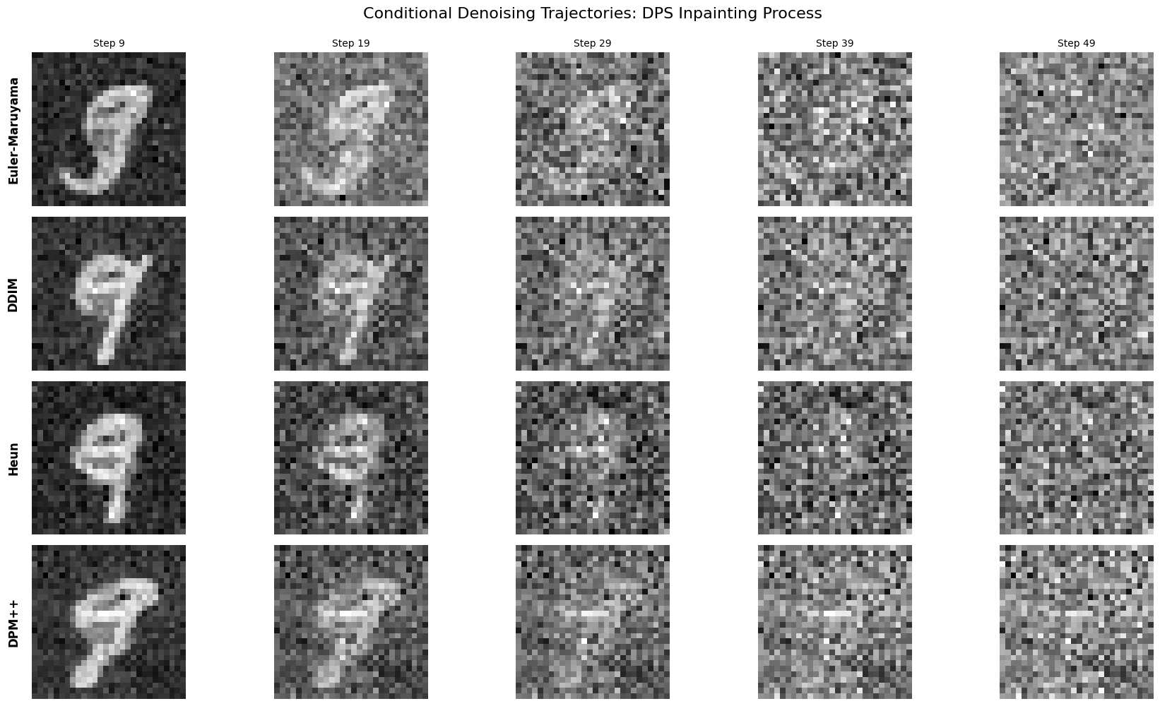
As we used the arguments keep_history=True we can visualize the entire sampling trajectory:

_images/539ec74da498144a5c6a21c37fc88af41b75d18ee1b148b8422efe02bacde54e.png

Now that we’ve seen unconditional generation, let’s tackle a more challenging task: solving inverse problems where we have partial observations and want to reconstruct the full image.

Conditional Generation: Solving Inverse Problems#

Conditional generation solves inverse problems where we want to generate \(x_0 \sim p(x_0|y)\) given measurements \(y = \mathcal{A}(x_0) + \epsilon\).

Example: Image Inpainting#

We’ll reconstruct masked MNIST digits using DPS (Diffusion Posterior Sampling) [Chung et al., 2023].

Think of DPS as a “guided” diffusion process:

Regular diffusion step: Move from noisy → less noisy using the learned model
Measurement correction: Check if the current estimate matches your observations (y)
Gradient guidance: Nudge the sample toward solutions that better match measurements

Mathematically:

Uses gradient of measurement likelihood: \(\nabla_x \log p(y|x_t)\)
Updates: \(x_{t-1} = \text{step}(x_t, t) - \gamma \nabla_x \|y - \mathcal{A}(x_t)\|^2\) where \(\text{step}(x_t, t)\) is the unconditional integrator step

The zeta parameter controls how strongly we enforce measurement consistency:

Too high → overfits to measurements, artifacts
Too low → ignores measurements, poor reconstruction

This is easily implemented in our framework as everything is modular:

@dataclass
class DPSDenoiser(CondDenoiser):
    epsilon: float = 1e-3  # Small constant to avoid division by zero in norm calculation
    zeta: float = 1e-2
    def step(
        self,
        rng_key: PRNGKeyArray,
        state: CondDenoiserState,
        measurement_state: MeasurementState,
    ) -> CondDenoiserState:
        y_meas = measurement_state.y
        position_current = state.integrator_state.position
        t_current = self.integrator.timer(state.integrator_state.step)

        # Compute measurement loss and gradient at current position
        def measurement_loss(x: Array) -> Array:
            # Tweedie estimate: x̂_0 from x at time t
            denoised = self.model.tweedie(
                                        SDEState(x, t_current), 
                                        self.predictor.score).position
            # Measurement consistency loss: ||y - A(x̂_0)||²
            residual = y_meas - self.forward_model.apply(denoised, measurement_state)
            return jnp.sum(residual ** 2)

        # Compute loss value and gradient ∇_x ||y - A(x̂_0)||²
        loss_val, gradient = jax.value_and_grad(measurement_loss)(position_current)

        # Adaptive guidance scale, normalized by residual magnitude
        zeta = self.zeta / (jnp.sqrt(loss_val) + self.epsilon)

        # Take unconditional integrator step (works with any integrator)
        integrator_state_uncond = self.integrator(state.integrator_state, self.predictor)

        # Apply measurement correction: x_{i-1} = x'_{i-1} - ζ ∇_x ||y - A(x̂_0)||²
        position_corrected = integrator_state_uncond.position - zeta * gradient

        # Create next state with corrected position
        integrator_state_next = replace(integrator_state_uncond, position=position_corrected)
        state_next = replace(state, integrator_state=integrator_state_next)

        return state_next

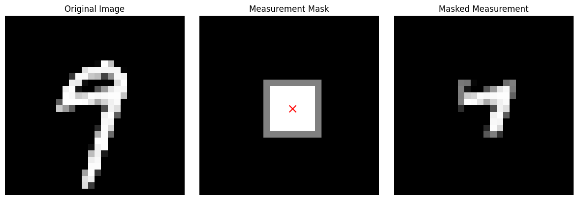
Let’s start with a square mask in the center of the image that selects which pixels are observed (1) and which are missing (0):

# Use a generated sample as test image
test_image = jnp.clip(results["DDIM"]["samples"][0], 0, 1)
# Create inpainting measurement
mask_model = SquareMask(size=8, img_shape=test_image.shape, std=0.1)
xi_center = jnp.array([14.0, 14.0])  # Center of 28x28 image
mask = mask_model.make(xi_center)
masked_image = test_image * mask

# Create measurement state
measurement_state = MeasurementState(y=masked_image, mask_history=mask)

print(f"Inpainting task: {jnp.mean(mask):.1%} visible, {jnp.mean(1 - mask):.1%} to reconstruct")

Inpainting task: 8.3% visible, 91.7% to reconstruct

_images/7f6026145beb4f5efc6fe9cdefd2a28a70b81edbabd223aebae4068eb2cedd61.png

Let’s create the DPSDenoiser with the EulerMaruyamaIntegrator and the mask_model as forward model \(\mathcal{A}\):

dps_euler_denoiser = DPSDenoiser(
    integrator=euler_maruyama,
    model=flow,  # The SDE/Flow model
    predictor=predictor,
    forward_model=mask_model,  # The measurement/masking operator
    x0_shape=img_shape,
    zeta=0.5,  # Guidance scale
)

All is needed to generate samples is to call the generate method of the DPSDenoiser instance with a random key and the number of samples we want.

# Generate conditional samples with DPS + Euler-Maruyama (showing the pattern)
n_cond_samples = 8

key_dps_euler = jax.random.PRNGKey(789)
state_dps_euler, history_dps_euler = dps_euler_denoiser.generate(
    key_dps_euler,
    measurement_state,  # Pass the measurement (masked image)
    n_steps,
    n_cond_samples,
    keep_history=True,
)

Now let’s generate samples with DPS using the other integrators (DDIMIntegrator, HeunIntegrator, DPMpp2sIntegrator) and compare both the generated samples and denoising trajectories.

_images/47c74c4459818cc3d5e4b9b87716c180ca760cdca91bb6f8362506270b1bb1e8.png

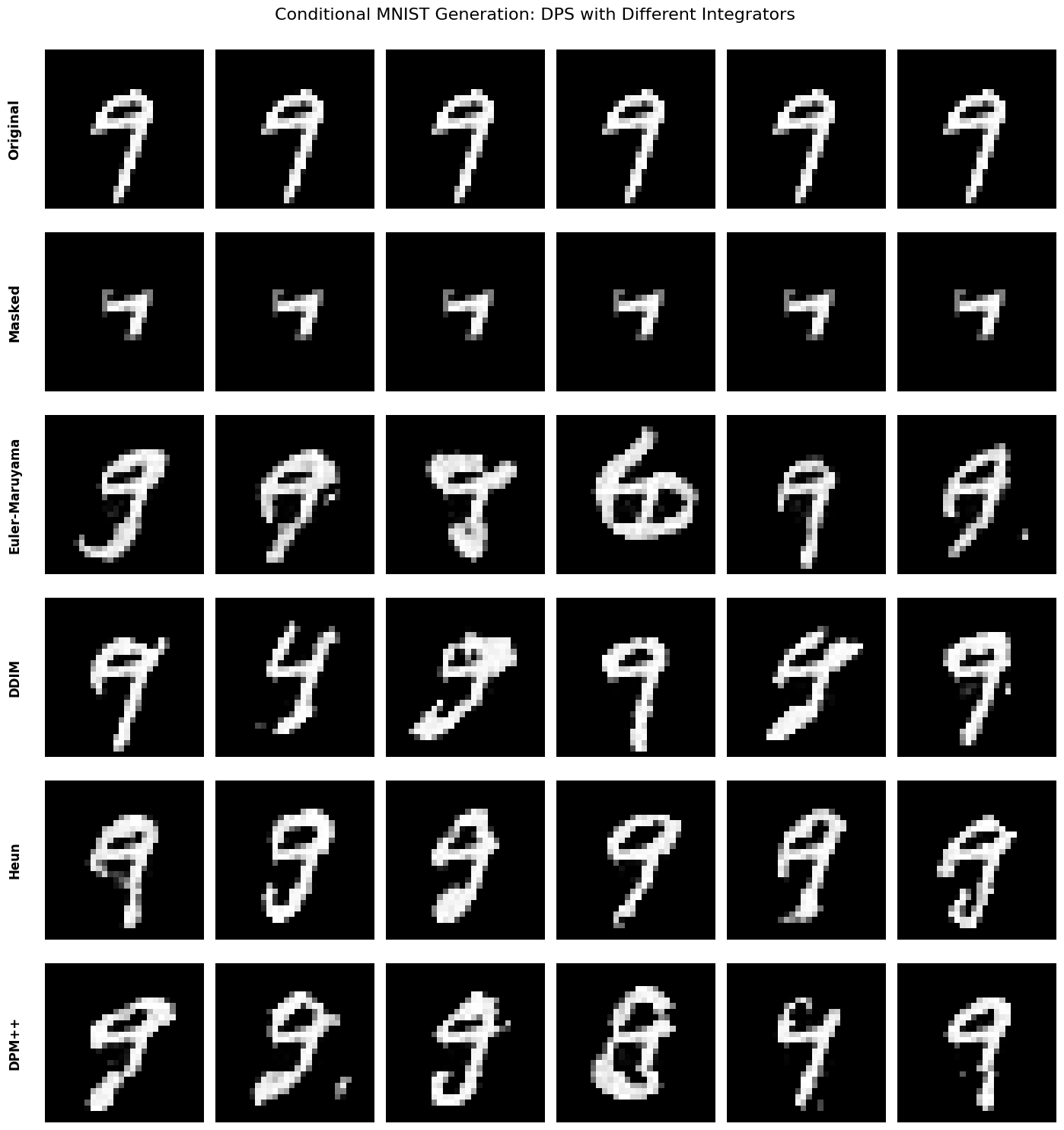
What to Look For: Conditional Generation#

Euler-Maruyama: May show more variation between samples (stochastic)
DDIM: Should produce clean, sharp digits
Heun/DPM++: Often highest quality, smoothest gradients

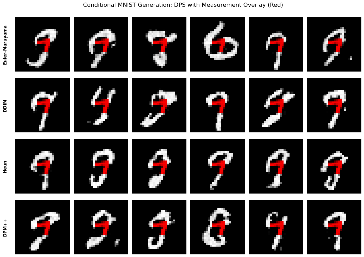
All methods should correctly preserve the central visible regions while plausibly reconstructing the outside of the center square.

_images/f3b1f51d422c9893f9c04d6390bae42c27216172fe64bb1cc453a97e6be39335.png

Verification: Measurement Consistency#

Let’s verify that the inpainted digits correctly preserve the conditioning measurements by overlaying them in red:

_images/08ab44d10df08e97112d319e8ebf59fbeee10afa1cbc98eda08499c34c368d34.png

Conclusion#

We showcased how different numerical integrators can be applied to unconditional and conditional diffusion sampling within a single modular framework.
This structure allows new solvers and conditioning operators to be incorporated easily, enabling rapid experimentation across a variety of inverse problems and data modalities.
The results illustrate how algorithmic choices—such as the integrator—directly shape sample diversity, fidelity, and computational cost, offering a practical foundation for extending diffusion models to real-world applications.

References#

[1] (1,2)

Hyungjin Chung, Jeongsol Kim, Michael T. Mccann, Marc L. Klasky, and Jong Chul Ye. Diffusion posterior sampling for general noisy inverse problems. In International Conference on Learning Representations (ICLR). 2023.

[2]

Xingchao Liu, Chengyue Gong, and Qiang Liu. Flow straight and fast: learning to generate and transfer data with rectified flow. In International Conference on Learning Representations (ICLR). 2023.

[3]

Cheng Lu, Yuhao Zhou, Fan Bao, Jianfei Chen, Chongxuan Li, and Jun Zhu. Dpm-solver++: fast solver for guided sampling of diffusion probabilistic models. arXiv preprint arXiv:2211.01095, 2022.

[4]

Jiaming Song, Chenlin Meng, and Stefano Ermon. Denoising diffusion implicit models. In International Conference on Learning Representations (ICLR). 2021.